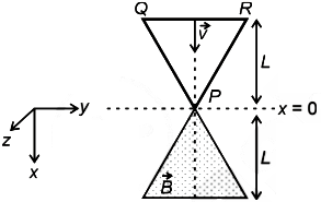
A region in the form of an equilateral triangle (in x-y plane) of height L has a uniform magnetic field 𝐵⃗ pointing in the +z-direction. A conducting loop PQR, in the form of an equilateral triangle of the same height 𝐿, is placed in the x-y plane with its vertex P at x = 0 in the orientation shown in the figure. At 𝑡 = 0, the loop starts entering the region of the magnetic field with a uniform velocity $\stackrel{\to <!--\; \to \; -->}{v}$ along the +x-direction. The plane of the loop and its orientation remain unchanged throughout its motion.

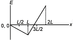
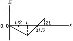
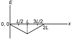
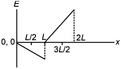
Which of the following graph best depicts the variation of the induced emf (E) in the loop as a function of the distance (x) starting from x = 0 ?

The correct option is Option 1 (represented by the graph in the first image, where the induced emf decreases linearly to a negative peak of magnitude $\frac{BLv}{\sqrt{3}}$ at $x=L$ and then increases linearly to a positive peak of magnitude $\frac{2BLv}{\sqrt{3}}$ at $x=2L$).

Step-by-Step Explanation:

1. Understanding the Geometry and Coordinate System:
From the given figure:
- The magnetic field region is an equilateral triangle of height $L$ with its vertex pointing in the $+x$-direction (downwards) starting at $x=0$.
- The conducting triangular loop $PQR$ has the same orientation (vertex $P$ pointing in the $+x$-direction) and moves in the $+x$-direction with uniform velocity $v$.
- At $t=0$, vertex $P$ is at $x=0$. Thus, the position of the vertex at time $t$ is $x=vt$.

For any point $x^{\prime }$ in the field region:
- The width of the magnetic field region is:

$w_{\text{field}}(x^{\prime })=\frac{2}{\sqrt{3}}{x}^{\prime }$

- For the loop with its vertex $P$ at position $x$, the distance from the vertex to any position $x^{\prime }$ is $x-x^{\prime }$. The width of the loop at $x^{\prime }$ is:

$w_{\text{loop}}(x^{\prime })=\frac{2}{\sqrt{3}}(x-x^{\prime })$

2. Case I: For $0\le x\le L$
The overlap of the loop with the magnetic field lies in the range $[0,x]$. The width of the overlapping region at any $x^{\prime }$ is limited by the narrower of the two regions:

$w_{\text{overlap}}(x^{\prime })=min(\frac{2}{\sqrt{3}}{x}^{\prime },\frac{2}{\sqrt{3}}(x-x^{\prime }))$

Evaluating the minimum, we split the integral at the midpoint $x^{\prime }=\frac{x}{2}$:

$A(x)=\frac{2}{\sqrt{3}}[{\int }_0^{x/2}{x}^{\prime }d{x}^{\prime }+{\int }_{x/2}^x(x-x^{\prime })d{x}^{\prime }]$

$A(x)=\frac{2}{\sqrt{3}}[\frac{x^2}{8}+\frac{x^2}{8}]=\frac{x^2}{2\sqrt{3}}$

The magnetic flux through the loop is:

$\Phi =BA(x)=\frac{B{x}^2}{2\sqrt{3}}$

The induced emf $E$ is:

$E=-\frac{d\Phi }{dt}=-\frac{d\Phi }{dx}v=-\frac{Bvx}{\sqrt{3}}$

Thus, for $0\le x\le L$, the emf $E$ decreases linearly with position $x$. At $x=L$:

$E(L)=-\frac{BLv}{\sqrt{3}}$

3. Case II: For $L\le x\le 2L$
In this region, the loop has partially exited the magnetic field. The overlapping region in the x-direction is now from $x^{\prime }=x-L$ to $x^{\prime }=L$.
The overlapping area is:

$A(x)=\frac{2}{\sqrt{3}}[{\int }_{x-L}^{x/2}{x}^{\prime }d{x}^{\prime }+{\int }_{x/2}^L(x-x^{\prime })d{x}^{\prime }]$

Calculating the integrals:

${\int }_{x-L}^{x/2}{x}^{\prime }d{x}^{\prime }=\frac{1}{2}[\frac{x^2}{4}-{(x-L)}^2]=-\frac{3}{8}$

${\int }_{x/2}^L(x-x^{\prime })d{x}^{\prime }={[x{x}^{\prime }-\frac{1}{2}}_{x/2}^L=-\frac{3}{8}$

Summing these gives:

$A(x)=\frac{2}{\sqrt{3}}$

Differentiating $A(x)$ with respect to $x$ to find the emf:

$E=-Bv\frac{dA}{dx}=-Bv\frac{2}{\sqrt{3}}(-\frac{3}{2}=\frac{Bv}{\sqrt{3}}(3x-4L)$

At the boundaries of this second interval:
- At $x=L$: $E(L)=-\frac{BLv}{\sqrt{3}}$ (continuous with Case I).
- At $x=2L$: $E(2L)=\frac{2BLv}{\sqrt{3}}$.
- The zero-crossing point is where $3x-4L=0\Rightarrow x=\frac{4}{3}L$.

Comparing the maximum magnitudes:
The positive peak value at $x=2L$ is exactly twice the magnitude of the negative peak at $x=L$.
This linear response and characteristic peak ratio matches the graph shown in Option 1.