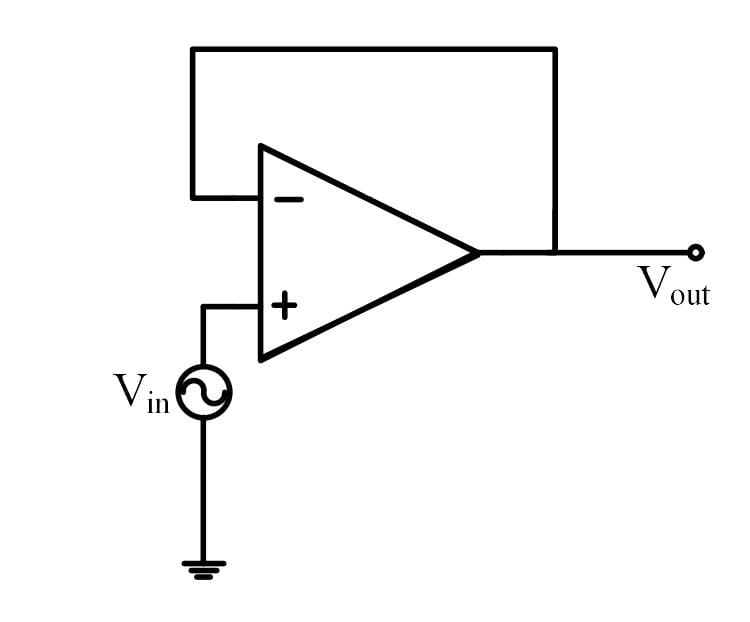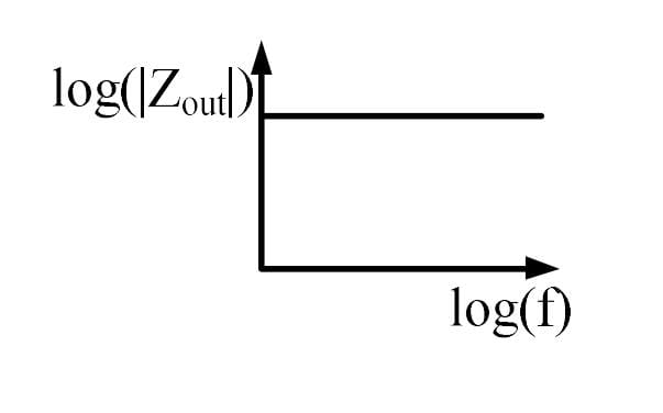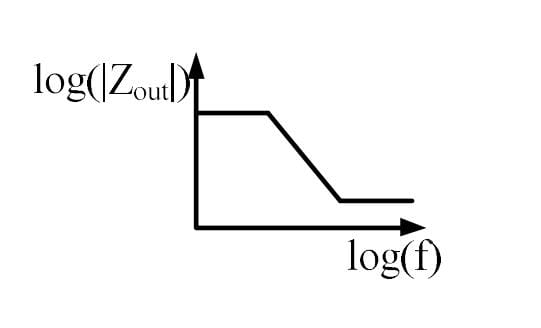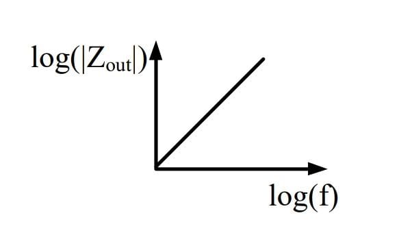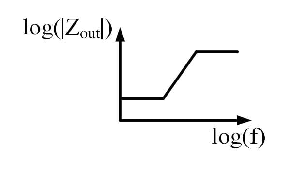
The output impedance of a non-ideal operational amplifier is denoted by Zout . The variation in the magnitude of Zout with increasing frequency, f , in the circuit shown below, is best represented by
Solution :
Correct Answer: The variation of with frequency is best represented by the curve in the option containing the graph that starts flat at a lower value, increases with a constant slope at intermediate frequencies, and then flattens out again at a higher value (corresponding to the image: WhatsApp Image 2024-09-30 at 2-1727688854245.jpeg).
Explanation and Step-by-Step Derivation:
1. Understanding the Circuit Configuration
The provided circuit diagram shows a non-inverting operational amplifier with its output terminal connected directly back to its inverting input terminal (). The input voltage is applied to the non-inverting terminal (). This configuration represents a negative feedback system known as a unity-gain buffer (or voltage follower). For this configuration, the feedback factor is:
2. Formula for Closed-Loop Output Impedance
In a negative feedback amplifier, negative feedback reduces the output impedance. The closed-loop output impedance is related to the open-loop output resistance and the open-loop gain by the relation:
Since , this simplifies to:
3. Modeling the Frequency Dependence of the Open-Loop Gain
A practical, internally compensated operational amplifier has an open-loop gain that rolls off at high frequencies. This behavior is typically modeled as a single-pole low-pass transfer function:
where is the DC open-loop gain (which is very large, typically in the range of to ) and is the open-loop corner (cutoff) frequency (typically around ).
4. Deriving the Closed-Loop Output Impedance
Substitute the expression for into the output impedance formula:
5. Analysis of Frequency Regions
To determine the shape of the magnitude graph in a log-log plot (i.e., versus ), we evaluate three distinct frequency ranges:
Case I: Low Frequencies ()
Here, the frequency term is extremely small compared to , so . The output impedance becomes:
Since is a constant value, the output impedance is constant and independent of frequency in this region. This corresponds to the flat plateau at low frequencies.
Case II: Intermediate Frequencies ()
In this region, the frequency is much larger than the corner frequency , meaning , so the numerator's imaginary term dominates over 1. However, is still significantly smaller than the open-loop gain , so the denominator is dominated by :
Taking the magnitude of both sides:
Taking the logarithm:
This represents a straight line with a slope of (equivalent to ). Thus, the magnitude of output impedance increases linearly with frequency in this range.
Case III: High Frequencies ()
At very high frequencies, the term becomes much larger than both 1 and . The imaginary terms dominate in both the numerator and the denominator, leading to:
Thus, the magnitude of the output impedance levels off at a constant value equal to the open-loop output resistance , resulting in another flat horizontal region at a higher impedance value.
Conclusion
Combining the three regions, the log-log plot of vs frequency begins flat at a low impedance level (), increases linearly with a slope of at intermediate frequencies, and then flattens out at a higher value (). This is accurately depicted in the plot shown in the fourth option.
Completely free for students. Educators & coaching institutes get 2 months free Pro trial to create tests.
Access unlimited practice questions, detailed step-by-step solutions, and exam study materials — completely free for students.
Create and conduct professional online assessments with AI question generation, tab proctoring, and comprehensive batch management.

Prepare effectively for GATE 2026 Electronics & Communication Engineering (EC) with this comprehensive Question Paper with Solutions. This resource includes detailed explanations, concept-wise solutions, previous year paper analysis, and exam-oriented practice to help aspirants strengthen core subjects like Electronic Devices, Analog Circuits, Digital Circuits, Signals & Systems, Network Theory, Control Systems, Electromagnetics, Communications, and more. Perfect for revision, self-assessment, and boosting your GATE 2026 EC preparation strategy.

Prepare for GATE 2026 Civil Engineering with the latest question papers, previous year papers, detailed solutions, syllabus, exam pattern, preparation tips, mock tests, and subject-wise study material. Download GATE 2026 CE question papers with solutions in PDF format and boost your preparation for top engineering institutes and PSU recruitment.
Copyright © 2026 Combe Labs Private Limited. All Rights Reserved.